Two ECUs at once

QInsight is not limited to a single device: in this example it measures, calibrates and stimulates two real ECUs at the same time — two NUCLEO-H723ZG boards connected to the PC through a switch. Each board gets its own driver and its own instance of the XCP on TCP protocol, and the signals of both units meet in one workspace: the graphs mix them on purpose, the tables keep each unit separate.

Each unit runs fully independently on its own IP address (192.168.2.20 and 192.168.2.21) — it generates three sine waves and accepts parameter writes. QInsight connects to each one with a separate XCP session, so an outage, calibration or stimulation of one unit never affects the other.

How it all works

1. Each board computes three sine waves. sine1 is split into raw (the internal model) and value (the published signal) — that pair demonstrates the STIM bypass. sine2 and sine3 are ordinary measurements.
2. Measured signals arrive through a 10 ms DAQ event, calibration parameters (amplitudes, periods) are read by 500 ms polling and can be written at any time.
3. A periodic script streams a slow sine into sine1_stim of both boards via STIM — with a different swing and frequency per unit, so the two boards are recognizable in the graphs at a glance.
4. With the sine1_bypass switch you choose independently per unit whether sine1_value is owned by the board's internal model or by the master through STIM.

The whole secret of a multi-unit project is in the configuration: one unit = one driver + one protocol instance; everything else (events, conversions, presentations) is shared.

The project step by step

Project and drivers

The project is called XCP on TCP - 2x Nucleo demo signals (STIM bypass).

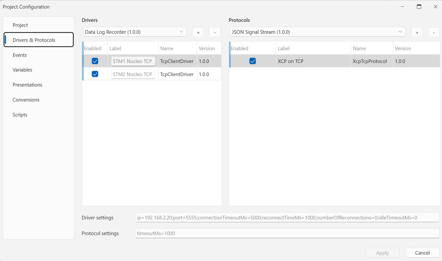
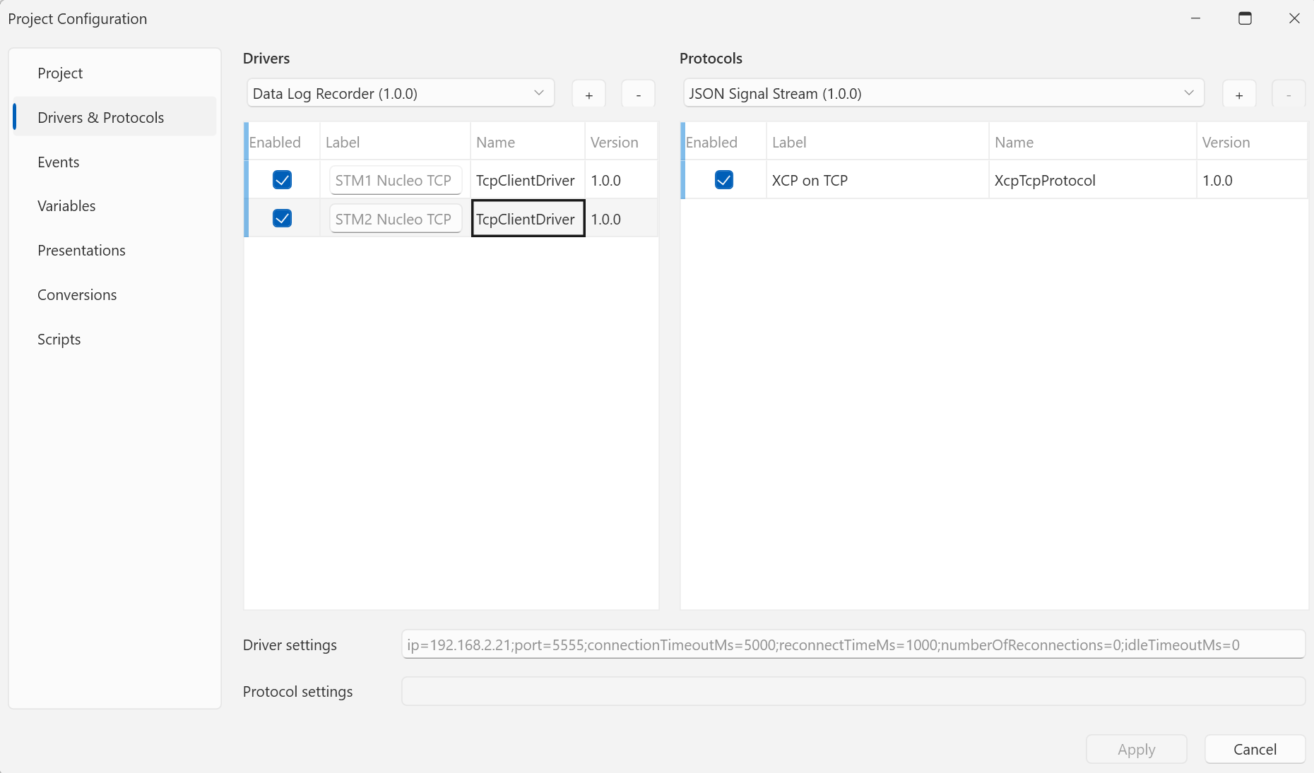
The Drivers & Protocols section holds two TCP Client drivers — STM1 Nucleo TCP and STM2 Nucleo TCP. Their settings are identical except for the IP address: STM1 points to 192.168.2.20, STM2 to 192.168.2.21. Under each driver runs its own instance of the XCP on TCP protocol — two independent XCP sessions, one per board.

Events

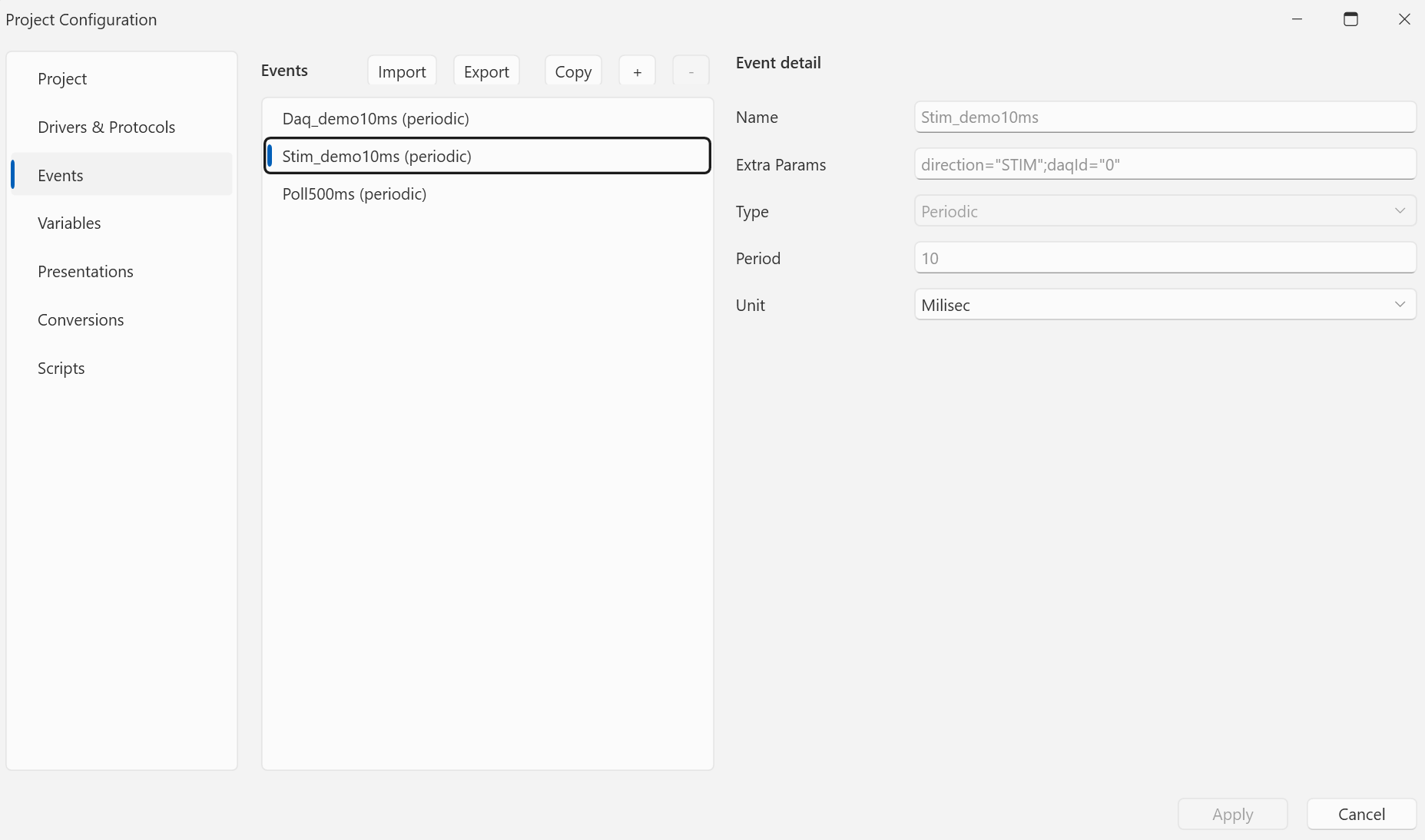
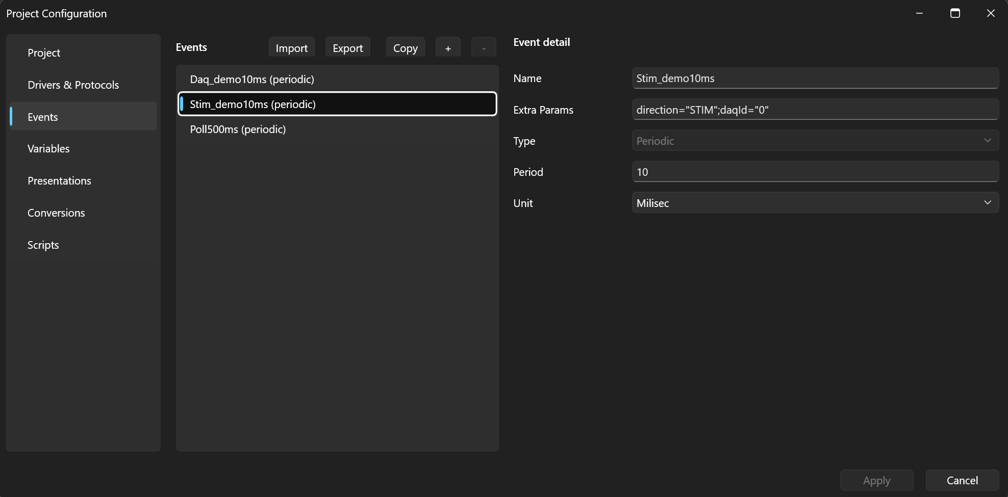
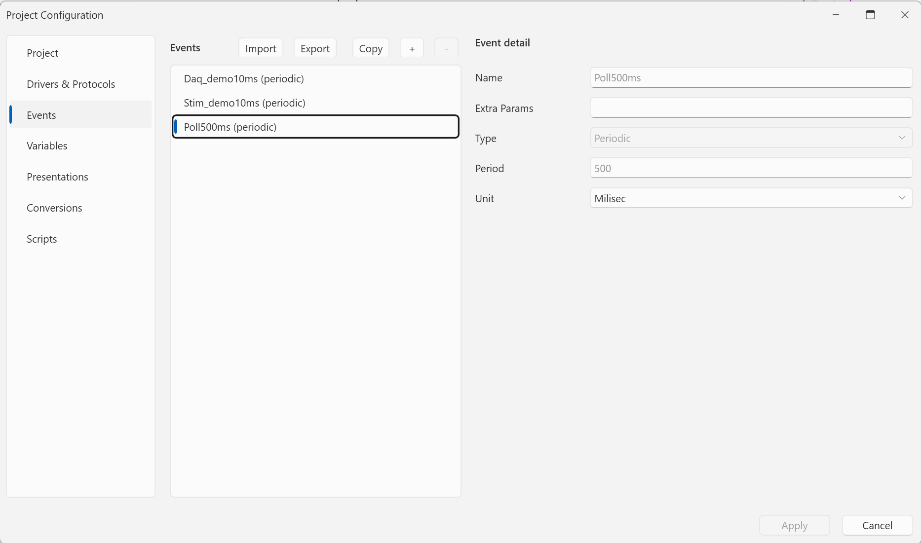
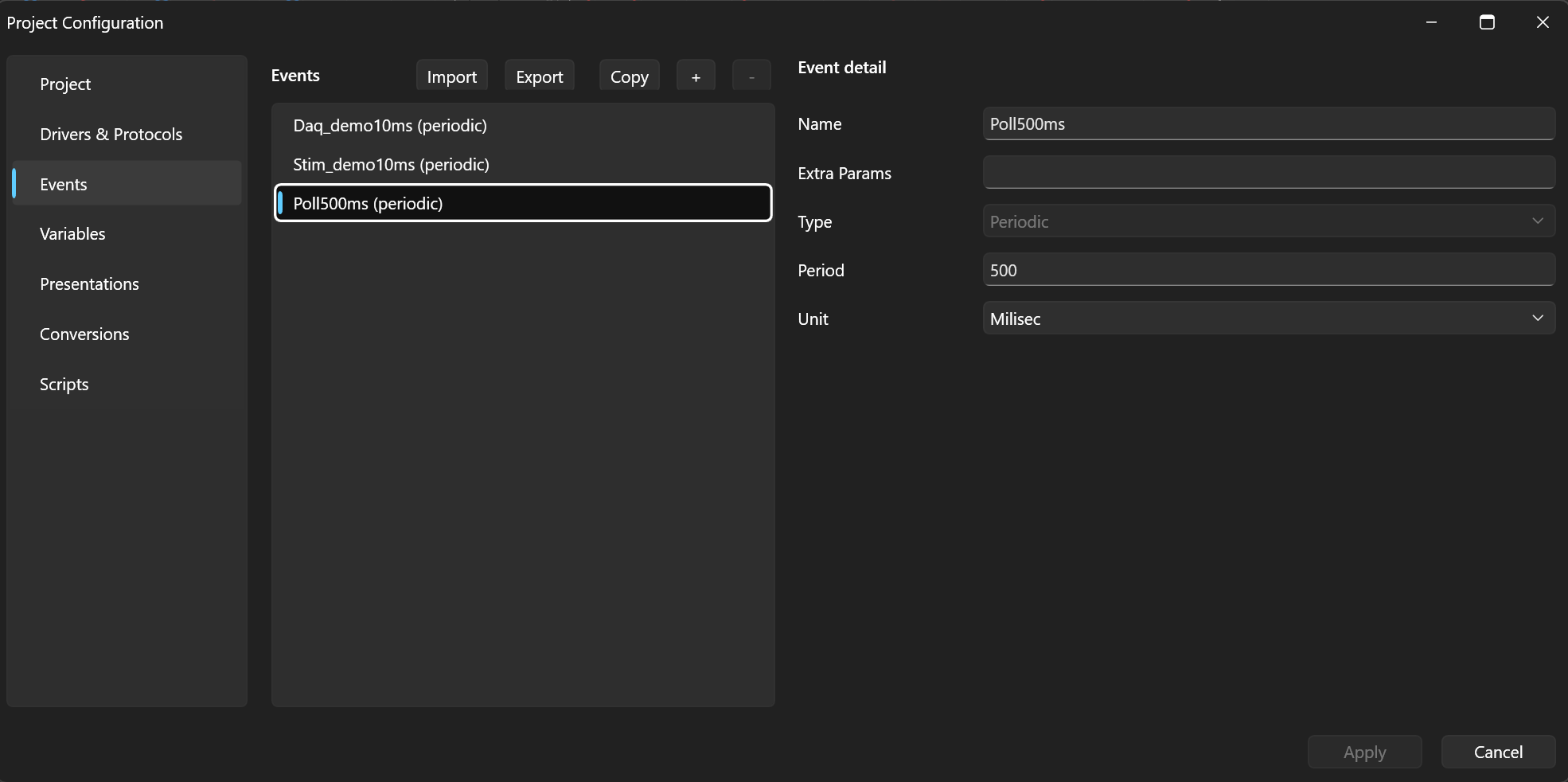
Three events defined once and shared by both protocols — each XCP session builds its own runtime context from them:

Conversions

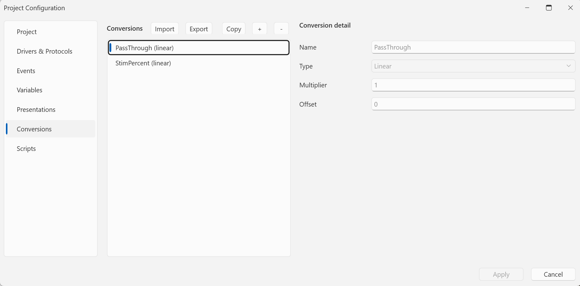
Two linear conversions: PassThrough (1:1) for most signals and StimPercent (eng = raw × 5 + 50) for the stimulation — the value is entered in percent of the ±10 range, so 75 % means raw 5.0. QInsight inverts the conversion on write and the STIM list streams the raw value.

Presentations

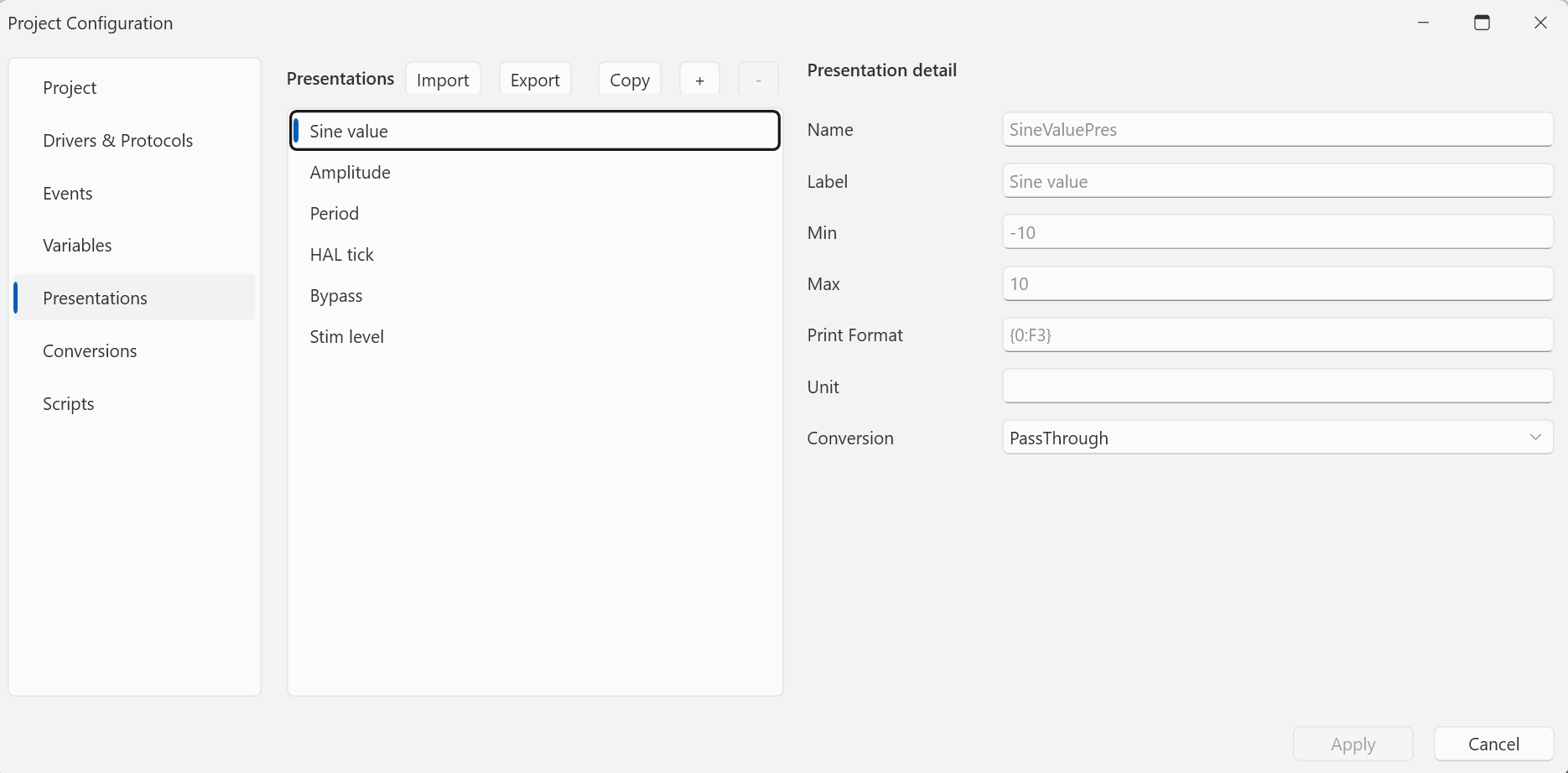
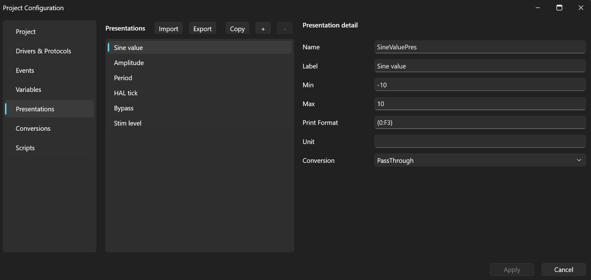
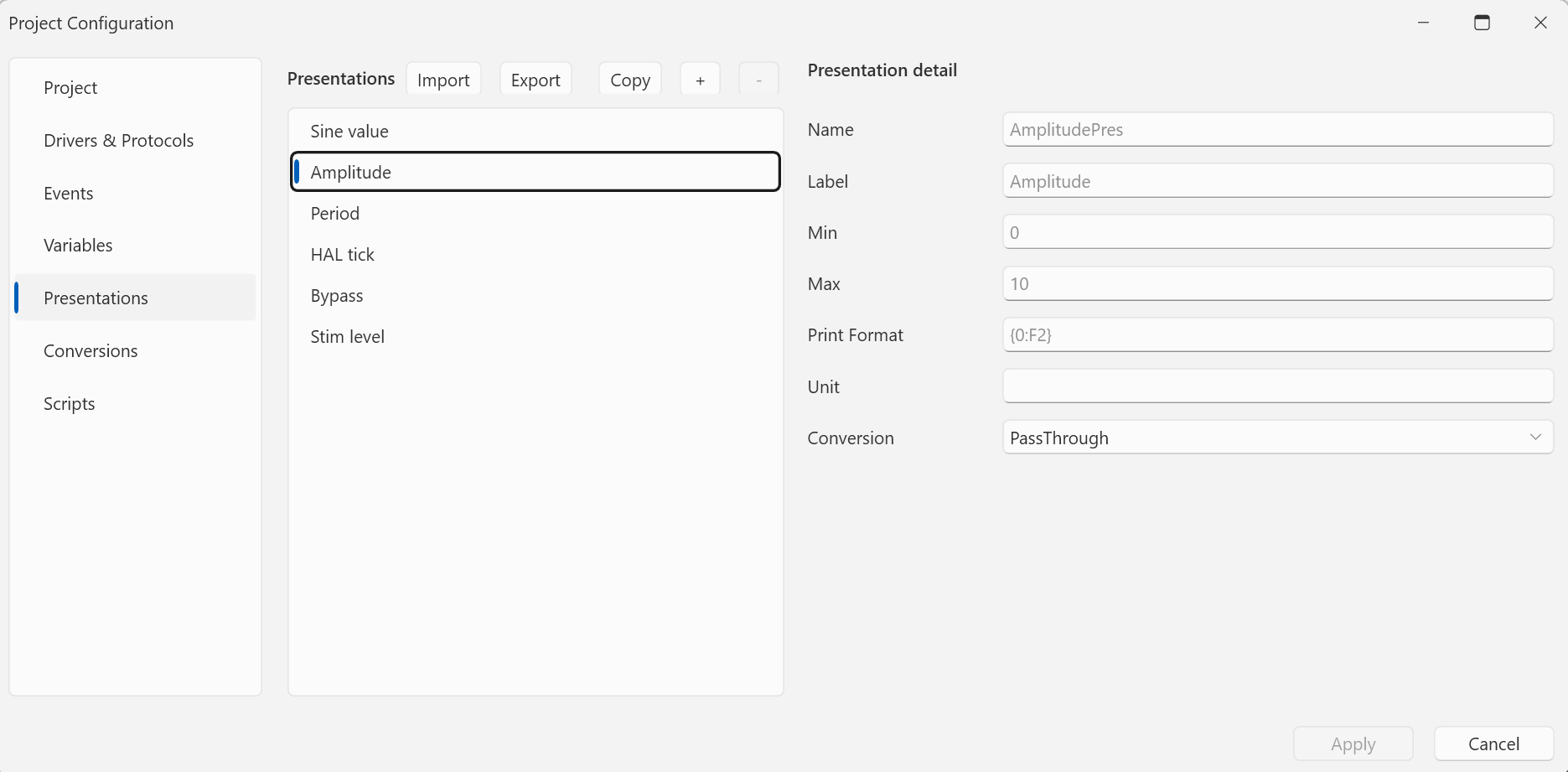
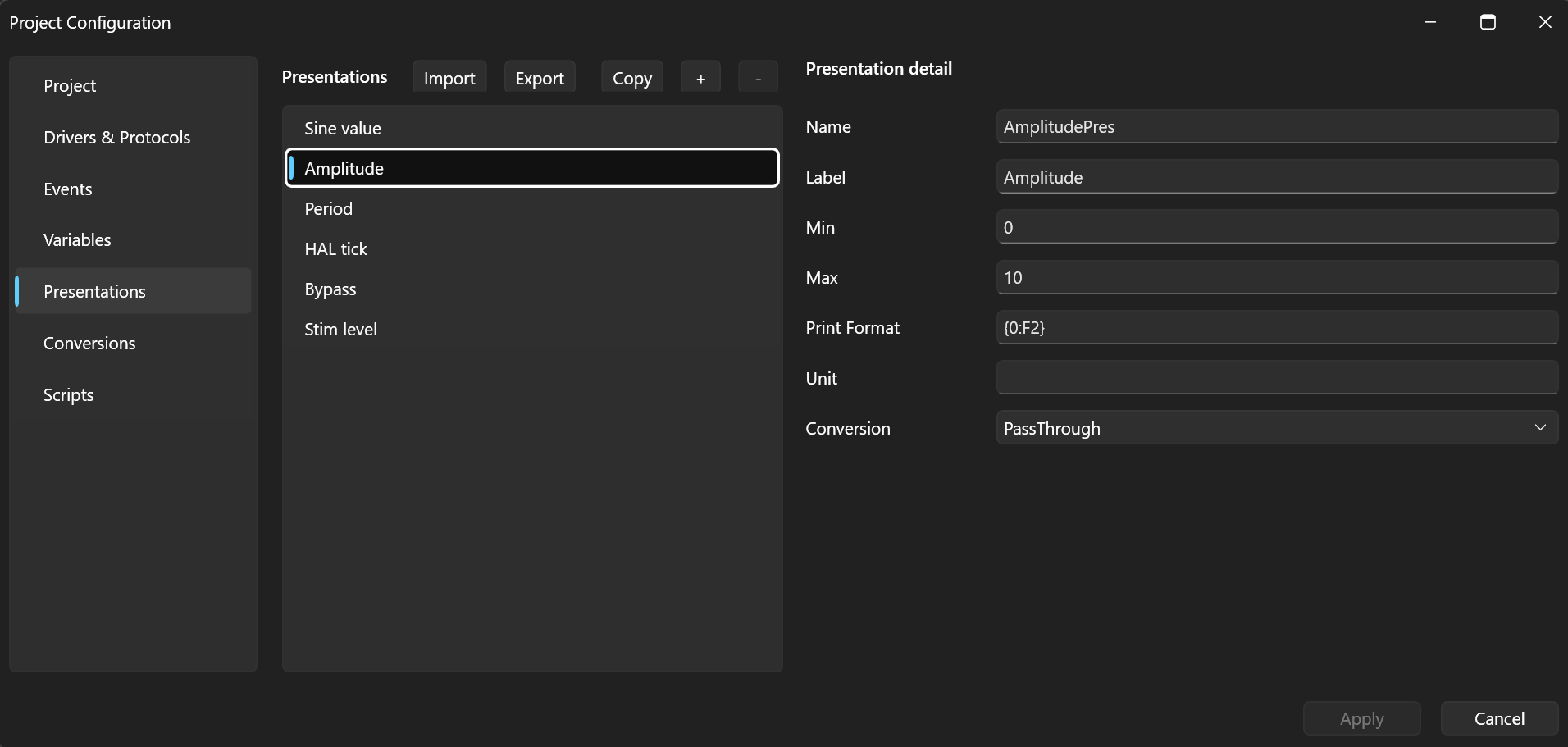
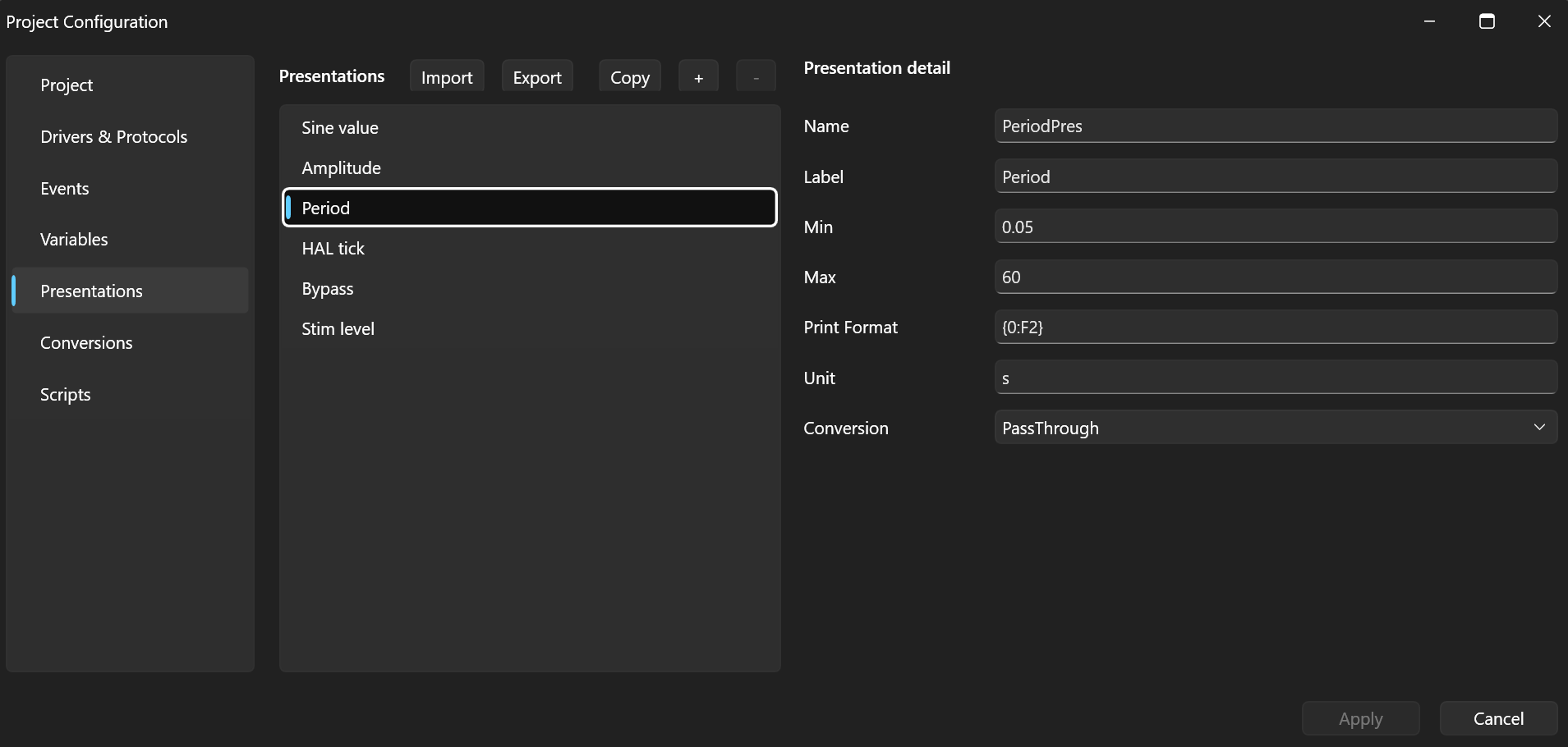
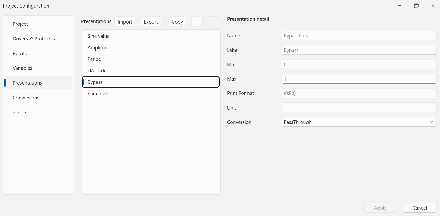
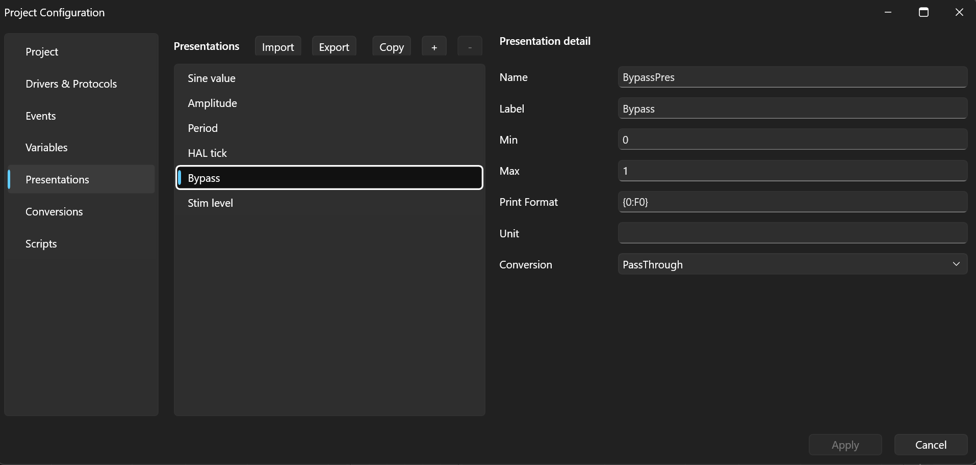
Six presentations matching the signal roles — and since both boards are identical, each presentation is shared by the STM1/STM2 pair of variables:

Variables

The project has 26 variables — the same set of thirteen, twice. The names carry the unit prefix (stm1_/stm2_), the namespaces split them into /Stm1 and /Stm2, and each half is bound to its own protocol — the twins differ only in which unit they belong to. The roles within each set of thirteen:

• sine1_value + sine1_raw — the published signal and the internal model (DAQ); the pair that shows the bypass.
• sine2_value, sine3_value — ordinary DAQ measurements.
• sine1–3_amplitude, sine1–3_period — writable calibration parameters, read by polling.
• uwTick (HAL tick) — the millisecond counter; proof that XCP reaches any global from the ELF.
• sine1_stim — a write variable streamed via STIM.
• sine1_bypass — the switch: 0 = the board owns the signal, 1 = the master does.

Scripts

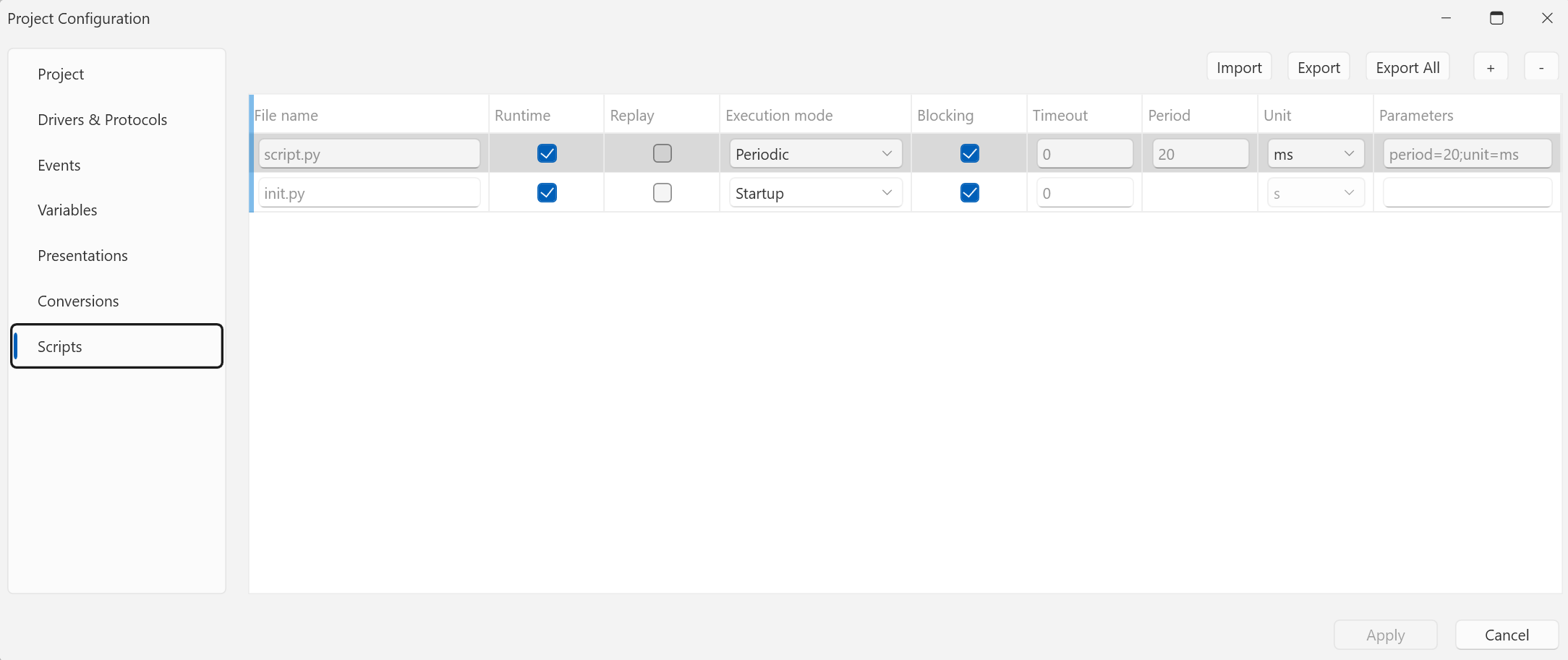
The stimulation is driven by a pair of scripts: init.py (Startup) prepares the parameters, script.py (Periodic, 20 ms) feeds both units at once — each with a different amplitude and frequency so the curves stay distinguishable in the graphs:

import math
t = 0
a = 50
b = 75
f1 = 1/8
f2 = 1/3

t += 0.02
stm1_sine1_stim.EngValue = 50 + a * math.sin(2 * math.pi * f1 * t)
stm2_sine1_stim.EngValue = 50 + b * math.sin(2 * math.pi * f2 * t)

STM1 gets a slow wave (8 s period), STM2 a faster one with a larger swing (3 s period). The writes are in percent through the StimPercent conversion — the script never deals with raw values.

The result

The workspace deliberately mixes signals of both boards in one graph: the left graph draws STM1 sine1 (value + raw, STIM bypass) together with STM2 sine2/3, the right one mirrors it — STM2 sine1 with STM1 sine2/3. Below the graphs sit two Watch Tables, one per unit, each with the complete set: values, writable calibration parameters, stimulation and bypass.

Switch STM1 Sine 1 bypass on and the dashed red curve in the left graph stops following the internal model — the slow scripted wave takes over while sine1_raw keeps running. STM2 is not affected at all. Calibration is just as independent: changing STM2 Sine 2 amplitude only shows on the second board.

What to take away

• More units = more driver + protocol pairs. Nothing else changes in the configuration; events, conversions and presentations are defined once and shared.
• The units run independently — each on its own address, with its own session; an outage of or a change to one never touches the other. Name prefixes and namespaces (/Stm1, /Stm2) keep the project tidy.
• Graphs are not tied to a source — signals from different devices go into one graph and get compared on a common time axis.
• Calibration and STIM stay per unit — each session has its own writes, its own bypass and its own stimulation; one script can drive all of them at once.

Next

• XCP on TCP — protocol and driver settings in the reference.
• XCP polling, DAQ, and STIM — how the three transfer modes differ and when to use which.
• Bit field and a script — another complete project-configuration example.