Simulation: all signals

The project Qenex_Sim_SimulData_AllSignals.qproj is in the Examples folder next to QInsight.exe. It needs no hardware: all data comes from the Simulation Signals protocol, which makes it the quickest way to try QInsight and to see most of the controls in action.

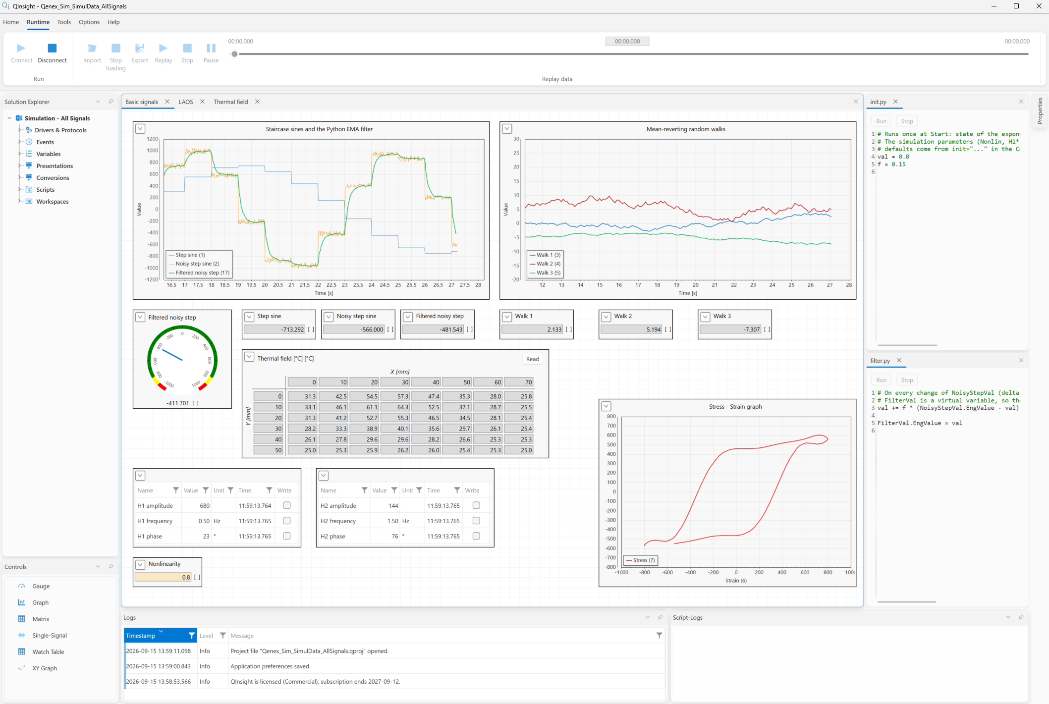
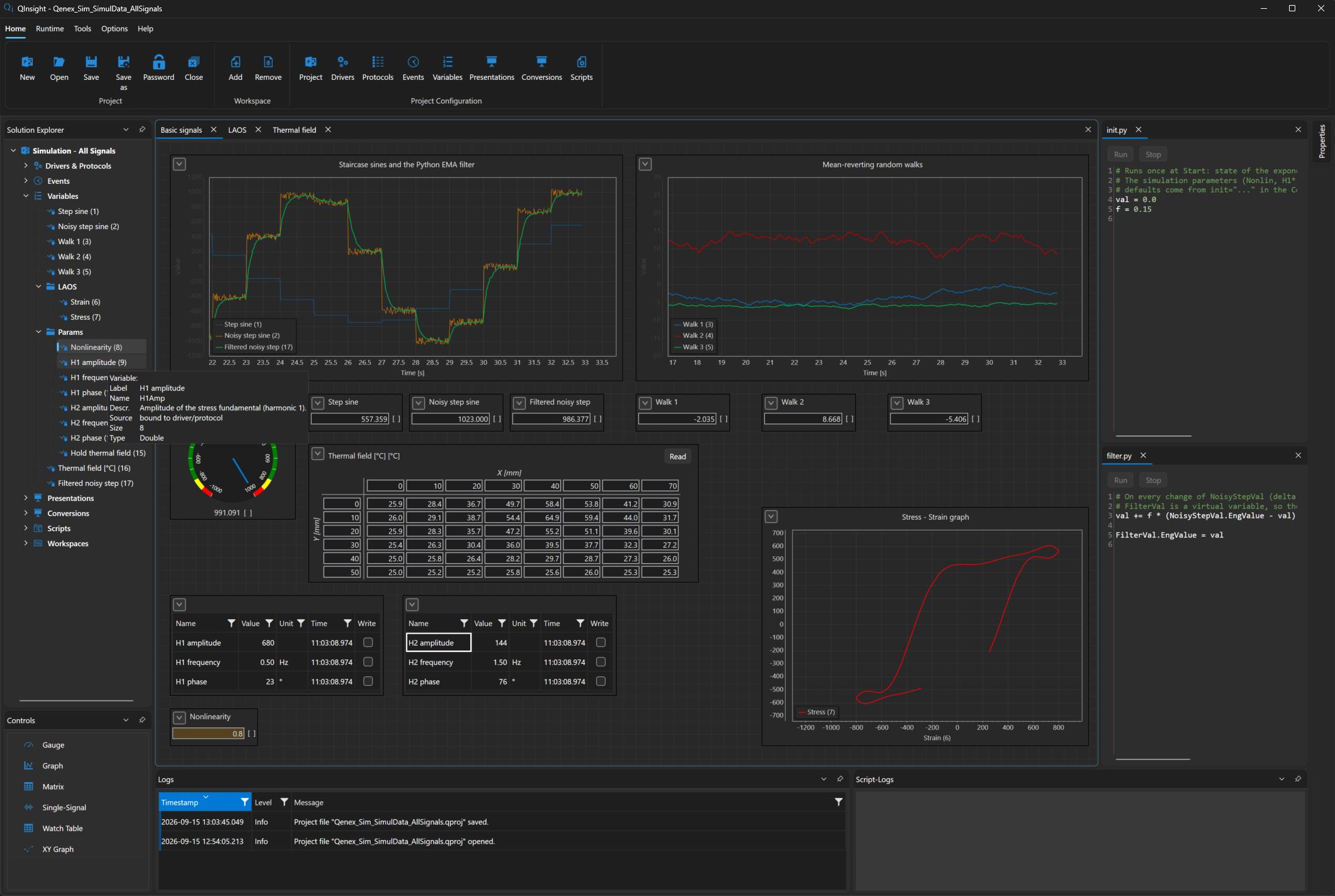
The Basic signals workspace while running

What the example shows

all seven scalar simulation signals (step, noisystep, walk1 to walk3, laosstrain, laosstress) and the thermal matrix signal,
a Python filter: an on-change trigger on the noisy signal runs a script that computes an exponential moving average and writes the result into a virtual variable, so the filtered curve is drawn next to the original,
the LAOS pair of strain and stress on a time graph and on an XY graph as a Lissajous loop, shaped live by the nonlinearity and harmonic parameters written from the watch table,
a thermal field as a Matrix variable in the Matrix control, with a Hold parameter that stops the generator and lets you edit cells,
parameter defaults through init= in the Comm params, without a script.

What you need

Just QInsight. Open the project, press Start and switch between the three workspace tabs.

The project

Drivers and protocols

Two pairs, neither with any settings:

Driver	Protocol	Role
Simulation	Simulation Signals	generates every signal and reads the parameters
Virtual Variables Host	Virtual Variables	publishes the script writes into `FilterVal` as samples

Events

Event	Period	Used by
`event20ms`	20 ms	staircase sines, the LAOS pair
`event100ms`	100 ms	random walks, parameters (the period plays no role there)
`event250ms`	250 ms	the thermal field

Variables

Generated signals (direction read):

Variable	Type	`signal`	Note
`StepVal`	float	`step`	staircase sine
`NoisyStepVal`	int	`noisystep`	filter input; on-change trigger `filter.py` (Delta 5, Eng)
`Walk1Val`, `Walk2Val`, `Walk3Val`	double	`walk1` … `walk3`	random walks around 0, 10 and −5
`LAOS/Strain`	double	`laosstrain`	`amp="800";freq="0.5"`
`LAOS/Stress`	double	`laosstress`	`amp="800";freq="0.5"`, nonlinearity from the parameter
`ThermalField`	Matrix 8×6, ushort	`thermal`	direction `readWrite`, `amp="40";freq="0.025"`, cells in °C (conversion 0.1), axes in mm

Parameters (direction write, not generated, read by the protocol):

Variable	`signal`	`init`	Meaning
`Params/Nonlin`	`nonlin`	0.6	stress nonlinearity, 0 to 2
`Params/H1Amp`	`h1amp`	680	amplitude of the fundamental
`Params/H1Freq`	`h1freq`	0.5 Hz	frequency of the fundamental, drives the strain too
`Params/H1Phase`	`h1phase`	23°	phase of the fundamental
`Params/H2Amp`	`h2amp`	144	amplitude of the 3rd harmonic
`Params/H2Freq`	`h2freq`	1.5 Hz	frequency of the 3rd harmonic
`Params/H2Phase`	`h2phase`	76°	phase of the 3rd harmonic
`Params/Hold`	`hold`	0	1 = freeze the thermal field

The project deliberately has no parameters for the 5th and 7th harmonic: their amplitude stays under the control of the nonlinearity, so a change of Nonlin is visible on the graph. With h3amp and h4amp present they would take precedence and Nonlin would have nothing left to act on.

The virtual variable FilterVal (double) is assigned to the Virtual Variables protocol; its Comm params are empty.

Scripts

init.py (mode Startup) only prepares the filter state. The simulation parameters are not set here: the protocol sets their defaults from init=.

val = 0.0
f = 0.15

filter.py (mode On Value Changed, triggered by NoisyStepVal) is the whole filter:

val += f * (NoisyStepVal.EngValue - val)

FilterVal.EngValue = val

It is an exponential moving average: the new value moves towards the measurement by the fraction f of the remaining distance. A smaller f means a smoother but lazier curve. The state val lives in a Python variable that all scripts of the project share. The write into FilterVal is published as a new sample because it is a virtual variable; a write into a variable of another protocol would raise no UI event.

Workspaces

Tab	Controls
Basic signals	graph of the staircase sines with the filter, graph of the random walks, a gauge and signal controls, plus the LAOS XY graph, the thermal-field matrix and watch tables of the H1 and H2 parameters as an overview of everything on one canvas
LAOS	time graph of strain (left axis) and stress (right axis), XY graph of stress against strain, a watch table of `Nonlin`, H1 and H2 in write mode, signal controls
Thermal field	the `ThermalField` Matrix control, a watch table with `Hold`

What you will see and what to try

After Start every control is emptied and fills with values read from the simulation; the stress oscillates with an amplitude of about ±580 and the XY graph draws a closed loop.

Parameters are written in the watch table in the row's write mode: the entered value is sent by the row's Write button (or by Enter when Write on Enter is on in the context menu). The effect shows in the graphs at once; the watch table shows the written value only after it is read back from the simulation (controls show read values, never written ones).

Filter: on the Basic signals graph watch the green filtered curve chase the orange noisy signal. Change f in init.py to 0.05 and restart the runtime: the filter gets smoother but slower.
LAOS: in the watch table write Nonlin = 0 and the loop turns into an ellipse; 1.5 deforms it. H2Amp = 300 bends the loop into an S, H1Phase = 90 opens it. H1Freq = 1 speeds up strain and stress together and the loop stays closed.
Thermal field: the hot spot orbits the plate centre once per 40 s. Write Hold = 1, switch the Matrix control to write mode, edit a cell and send it with the Write button (or Enter with Write on Enter on); the value stays until Hold goes back to 0.
Matrix axes: edit a value on the X axis. The generator never rewrites the axes, so the edit survives even with Hold = 0.
Stop and Start: the simulation restarts from zero, the filter from val = 0, and the parameters return to their init= values.

Simulation Signals and Virtual Variables in the protocol reference
Accessing variables from a script
Matrix variable
Controls
Bit field and a script — another example with virtual variables and an on-change trigger